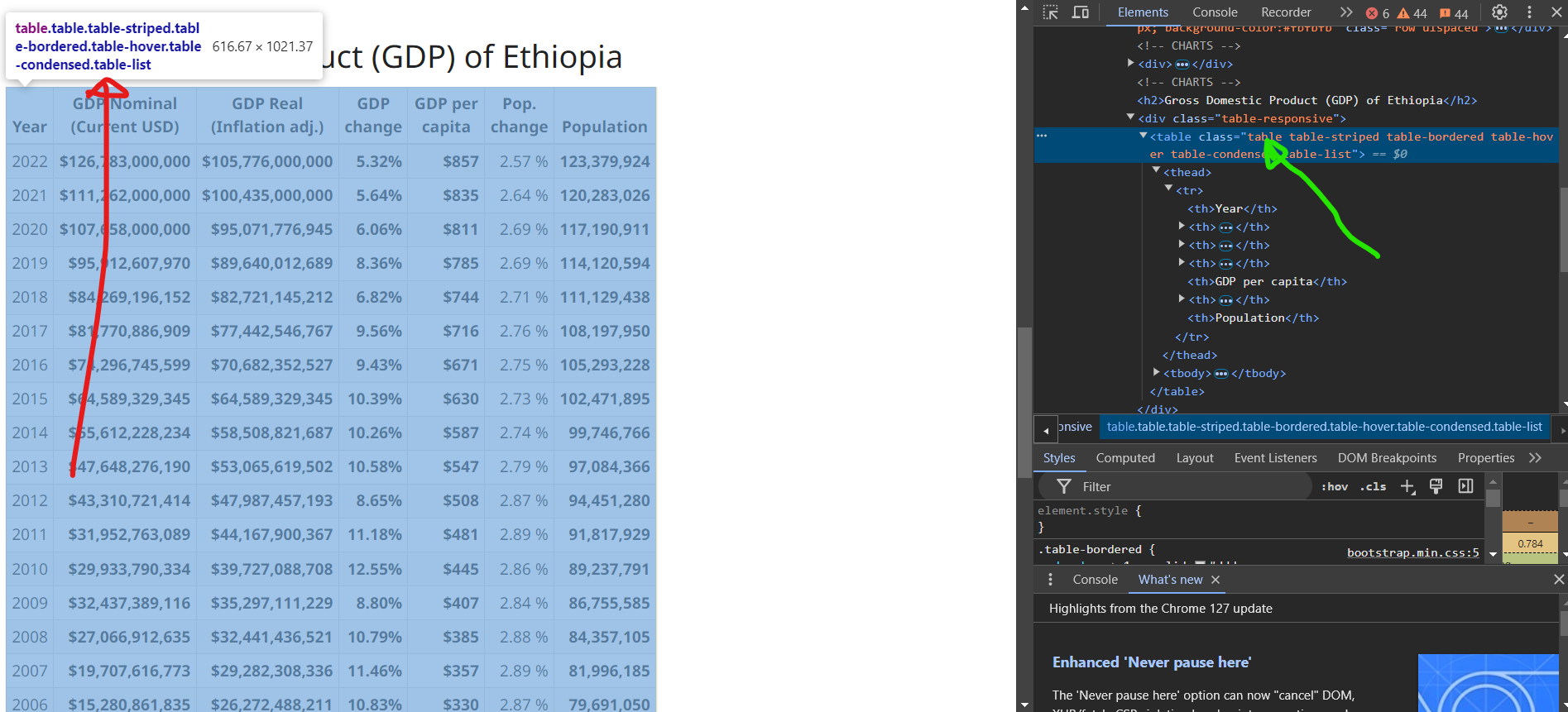
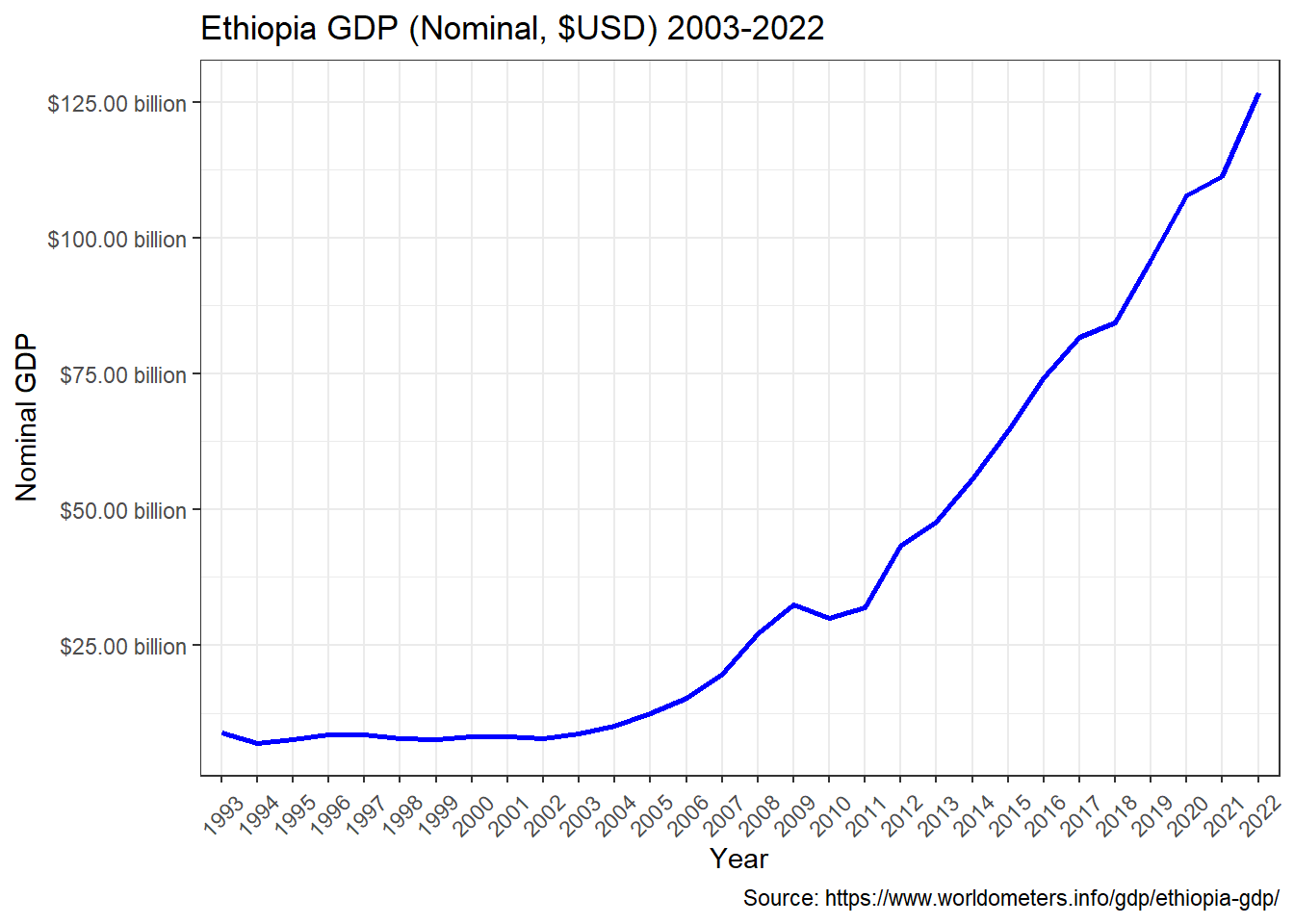
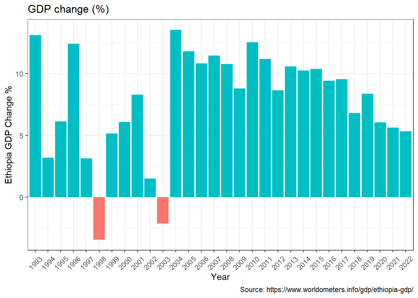
Web Scraping in R: Import table directly from website

web scraping
rvest
ggplot2
Author

Gutama Girja Urago

Published

May 20, 2024

What and why?

In this blog, we are going to import table from website into R. This is very important because it saves a time to copy the table manually and going through a lot of pain in excel to import the table into R. Doing it in that way is time consuming, tedious and prone to mistake. That’s why rvest (harvest) package is there for you on CRAN. Install the package from CRAN using install.packages() function and let’s dive in.

Web Scrapping

First we need to have the url for the website from which we are planning to import the data as a dataframe in R. Here I am using Ethiopian GDP table from worldmeters website. Once we have the link to the website, we have to load the package and read html file from that page of website, which also contains the table of interest.

# install.packages(rvest)         # Install the package if you do

library(rvest)

tbl_url <- "https://www.worldometers.info/gdp/ethiopia-gdp/"

raw_html <- read_html(tbl_url)


raw_html
{html_document}
<html lang="en">
[1] <head>\n<meta http-equiv="Content-Type" content="text/html; charset=UTF-8 ...
[2] <body>\n<!-- Google tag (gtag.js) --><script async src="https://www.googl ...

The above HTML content contains two main parts: the head and the body. The body part of the document typically contains the content of interest. HTML documents are usually styled using CSS, and the CSS selector helps us pick specific elements that we are interested in. To find the CSS of the element that we are interested in, right-click on the element of interest on the web and select inspect. Next, move your mouse over the codes in the Elements section until it highlights all parts of the table in blue.

There are two widely used CSS selectors, namely, class and id. One HTML element can have multiple classes. In this case, a table is one of the class selectors. Whenever you use the class selector, put a dot (.) before the class name. The precise CSS selector is the code that appears at the top of the table (shown by a red arrow), but it requires a significant amount of time to write. So, let’s start with the first class name, which is table. We could have also used xpath instead of CSS to select an element, but let’s keep it aside for now.

element <- html_elements(raw_html, css = ".table")
element
{xml_nodeset (1)}
[1] <table class="table table-striped table-bordered table-hover table-conden ...

Once you select the element, it’s still in HTML format and hard to understand. So, let’s convert it into an R object. Now, we see that there are actually two table objects in the returned HTML.

tables <- html_table(element)
tables
[[1]]
# A tibble: 30 × 7
    Year `GDP Nominal (Current USD)` `GDP Real  (Inflation adj.)` `GDP change`
   <int> <chr>                       <chr>                        <chr>       
 1  2022 $126,783,000,000            $105,776,000,000             5.32%       
 2  2021 $111,262,000,000            $100,435,000,000             5.64%       
 3  2020 $107,658,000,000            $95,071,776,945              6.06%       
 4  2019 $95,912,607,970             $89,640,012,689              8.36%       
 5  2018 $84,269,196,152             $82,721,145,212              6.82%       
 6  2017 $81,770,886,909             $77,442,546,767              9.56%       
 7  2016 $74,296,745,599             $70,682,352,527              9.43%       
 8  2015 $64,589,329,345             $64,589,329,345              10.39%      
 9  2014 $55,612,228,234             $58,508,821,687              10.26%      
10  2013 $47,648,276,190             $53,065,619,502              10.58%      
# ℹ 20 more rows
# ℹ 3 more variables: `GDP per capita` <chr>, `Pop. change` <chr>,
#   Population <chr>

It is stored as a list, let extract it and the rest is cleaning.

gdp_tbl <- tables[[1]] 
gdp_tbl
# A tibble: 30 × 7
    Year `GDP Nominal (Current USD)` `GDP Real  (Inflation adj.)` `GDP change`
   <int> <chr>                       <chr>                        <chr>       
 1  2022 $126,783,000,000            $105,776,000,000             5.32%       
 2  2021 $111,262,000,000            $100,435,000,000             5.64%       
 3  2020 $107,658,000,000            $95,071,776,945              6.06%       
 4  2019 $95,912,607,970             $89,640,012,689              8.36%       
 5  2018 $84,269,196,152             $82,721,145,212              6.82%       
 6  2017 $81,770,886,909             $77,442,546,767              9.56%       
 7  2016 $74,296,745,599             $70,682,352,527              9.43%       
 8  2015 $64,589,329,345             $64,589,329,345              10.39%      
 9  2014 $55,612,228,234             $58,508,821,687              10.26%      
10  2013 $47,648,276,190             $53,065,619,502              10.58%      
# ℹ 20 more rows
# ℹ 3 more variables: `GDP per capita` <chr>, `Pop. change` <chr>,
#   Population <chr>

Cleaning the Data

Below we can see that all columns, except year, are stored as character because of dollar sign ($) and commas (,), which R doesn’t allow to happen.

gdp_tbl <- janitor::clean_names(gdp_tbl)


library(tidyverse)

glimpse(gdp_tbl)
Rows: 30
Columns: 7
$ year                    <int> 2022, 2021, 2020, 2019, 2018, 2017, 2016, 2015…
$ gdp_nominal_current_usd <chr> "$126,783,000,000", "$111,262,000,000", "$107,…
$ gdp_real_inflation_adj  <chr> "$105,776,000,000", "$100,435,000,000", "$95,0…
$ gdp_change              <chr> "5.32%", "5.64%", "6.06%", "8.36%", "6.82%", "…
$ gdp_per_capita          <chr> "$857", "$835", "$811", "$785", "$744", "$716"…
$ pop_change              <chr> "2.57 %", "2.64 %", "2.69 %", "2.69 %", "2.71 …
$ population              <chr> "123,379,924", "120,283,026", "117,190,911", "…

Let’s remove all unnecessary characters and convert to numeric with a short function.

convert_to_numeric <- function(x) {
  as.numeric(str_remove_all(x, "[$,%\\s]"))
}

gdp_tbl <- gdp_tbl |> 
        mutate_all(convert_to_numeric)

glimpse(gdp_tbl)
Rows: 30
Columns: 7
$ year                    <dbl> 2022, 2021, 2020, 2019, 2018, 2017, 2016, 2015…
$ gdp_nominal_current_usd <dbl> 126783000000, 111262000000, 107658000000, 9591…
$ gdp_real_inflation_adj  <dbl> 105776000000, 100435000000, 95071776945, 89640…
$ gdp_change              <dbl> 5.32, 5.64, 6.06, 8.36, 6.82, 9.56, 9.43, 10.3…
$ gdp_per_capita          <dbl> 857, 835, 811, 785, 744, 716, 671, 630, 587, 5…
$ pop_change              <dbl> 2.57, 2.64, 2.69, 2.69, 2.71, 2.76, 2.75, 2.73…
$ population              <dbl> 123379924, 120283026, 117190911, 114120594, 11…

Making a Graph

With a minimal code, we can produce the same graph and customize the way we want.

gdp_tbl |> 
        ggplot() + 
        geom_line(aes(x = factor(year), 
                      y = gdp_nominal_current_usd,
                      group = 1),
                  color = "blue", linewidth = 1) + 
        scale_y_continuous(labels = scales::dollar_format(
          scale = 1/1000000000,
          suffix = " billion")) +
 
        labs(x = "Year",
             y = "Nominal GDP",
             title = "Ethiopia GDP (Nominal, $USD) 2003-2022",
             caption = "Source: https://www.worldometers.info/gdp/ethiopia-gdp/") + 
        theme_bw() + 
        theme(axis.text.x = element_text(angle = 45, vjust = 0.5))

Here is the second graph as well.

gdp_tbl |>
  mutate(growth = ifelse(gdp_change > 0, "positve", "negative")) |> 
  ggplot(aes(x = factor(year), y = gdp_change, fill = growth)) + 
  geom_col() + 
  labs(title = "GDP change (%)",
       y = "Ethiopia GDP Change %",
       x = "Year",
       fill = "",
       caption = "Source: https://www.worldometers.info/gdp/ethiopia-gdp/") +
  theme_bw() + 
  theme(axis.text.x = element_text(angle = 45, vjust = 0.5),
        legend.position = "none")